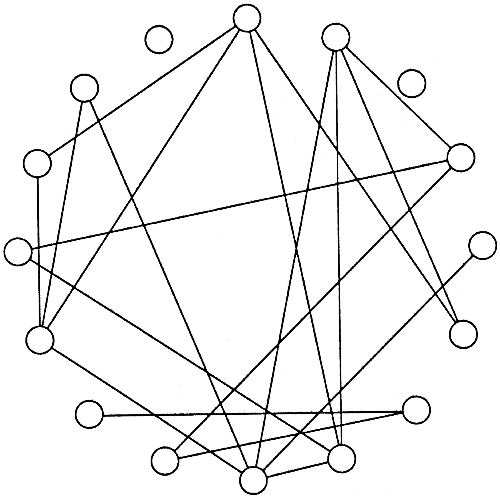
Humans have an intuitive sense of symmetry and aesthetics. We try our best to make it easy to understand the concept we’re trying to explain.

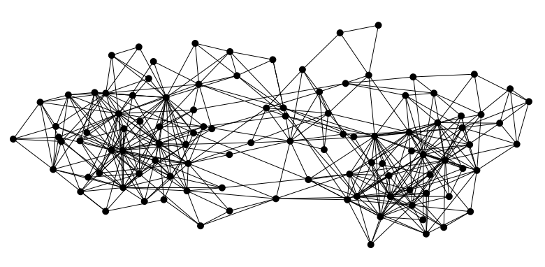
In textbooks, we see images like the one above, and not like this one..

I’m having labs in college where I have to implement various algorithms on graphs. The first step, however, was to draw one. The Random approach was the easiest. Randomly plot N Nodes anywhere in the screen, and connect them. If you’re lucky, your graph might look good. Mostly they didn’t.

There were people who tried this interesting approach: Given, N Nodes, arrange them in a Circle: with ‘360/N’ angular separation. Given the center, angle & radius can be easily converted to X, Y using basic trigonometry.

This was good. But we could do better. I searched for the best way to do this, and ended up reading this paper.

Anyway, The paper promised to take graphs from (a) to (b) using a method called Simulated Annealing.

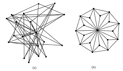
The paper defines the characteristics of a good drawing such as Evenly distributed nodes, edges having approximately the same lengths, minimal edge crossing, and Symmetry. Oh, and fitting snugly inside the window you’re drawing.

SA is derived from a Metallurgical process called Annealing, used to turn liquids to their crystalline form. Probability with which a system changes from one energy state to the next is

\(\\e^{-\frac{E_2 - E_1}{kT}}\)

This rule implied that whenever the energy E_2 of the candidate state is smaller than the current energy E_1 $, the system will take the move, else the state change is probabilistic.

A rough algorithm for SA is as follows:

Choose an initial configuration \(\sigma\) and an initial temperature \(T\)

Repeat the following (usually some fixed number of times):

1. Choose an initial configuration \(\sigma\) and an initial temperature \(T\)

2. Repeat the following (usually some fixed number of times):

   2.1 Choose new configuration \(\sigma’\) from the neighborhood of \(\sigma\)

   2.2 Let \(E\) and \(E’\) be the value of the cost function at \(\sigma\) and \(\sigma’\) respectively

   2.3 If \(E’\) < \(E\) or \(random(0,1) < e^{(E - E’)/T)}\) the set \(\sigma\) to \(\sigma’\).

   2.4 Decrease Temperature \(T\)

3. If Termination rule is satisfied, stop. else go back to step 2

The algorithm takes in an adjacency list representation of our graph, and should hopefully return coordinates of our graph nodes that look good. We chose an initial set of random coordinates for every node. Our energy function should be designed in such a way that a ‘nicer’ configuration should have a lower energy state. We talked about the characteristics of a good graph, but here are them again in detail.

Node distribution

Our nodes should be evenly spread across the window. Two components of the energy function take care of this. One to prevent nodes from getting too close. Second deals with window borders.

We add \(a_{ij}\) Energy function. if \(d_{ij}\) is the distance of node \(i\) to \(j\).

\(a_{ij} = \frac{\lambda_1}{d_{ij}^2}\)

This looks similar to the Electric Potential function. Lambda is a normalizing factor to define the importance of this particular criteria.

Window Edges

The energy function for Window Edges bases itself of the distance between node and Window Edges

\(m_i = \lambda_2 ( \frac{1}{r^2_i} + \frac{1}{l^2_i} + \frac{1}{t^2_i} + \frac{1}{b^2_i})\)

Where \(r_i\),\(l_i\),$t_i& $b_iare the distances of node i to right, left, top and bottom window edges. This ensures that nodes are prevented from getting too close to window border.

Edge lengths

we try to shorten edge lengths but not make the graph too crowded. For each edge k we add the term

\(c_k = \lambda_3d_{k}^2\)

These 3 criteria are enough for most graphs, but they won’t look good on all graphs. So we’ll take a look at edge crossings and node to edge distances

Edge crossing

We prevent edge crossing simply by adding an extra \(\lambda_4\) for every edge that crosses

Node to edge sides

Edges may get too close to a node. Mostly this is taken care by rest of the function, but adding this extra energy covers more cases

\(h_{kl} = \frac{\lambda_5}{g_{kl}^2}\)

There is an additional minimum distance rule in the paper, which I ignored for my code as it was working neatly without it. After every step of energy change, The temperature should be reduced. We follow this rule:

\(T' = \lambda T\)

with \(\lambda\) between 0.6 and 0.95.

Here is an 8x speedup video of my implementation on Turbo C++.

I did this mostly in a small laptop which didn’t belong to me at the time, and I hence lost most of the code. I’m looking forward to re implementing it here in Javascript so that anyone can play around with it :)